How to fix common errors in Excel

I’ll be the first to admit that not one of my students has ever looked overly enthused when I tell them they’re going to learn how to use worksheets in Microsoft Excel. There’s understandably even less enthusiasm—and downright frustration—when they’re forced to deal with back-to-back error messages. 

That’s when I swoop in with a handy cheat sheet to help fix common Excel errors. (When you teach a course on Excel, you take every “ooh!” and “aah!” where you can get it.) 

This is that cheat sheet. 

How to fix a #SPILL error in Excel

Before we dive into #SPILL! errors, let’s talk about spills. A spill in Excel means that a formula produces multiple values (also known as an array), and those values are automatically populated in the neighboring cells (also known as a spill range).

For example, the formula =UNIQUE(A2:A14) placed in cell D2 would pull every unique value from cells A2 to A14 and output them starting in cell D2. In this case, Excel would output nine unique ingredients, spilling down nine rows. 

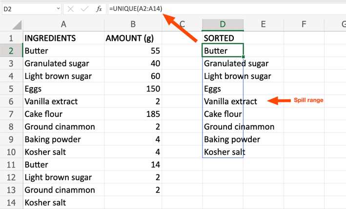
The spill range and the values within it change automatically (or dynamically) as the source data (in this case, cells A2 through A14) or the formula are updated. 

An Excel SPILL error occurs when a formula produces multiple values, but Excel can’t output one or more of these results. There are many reasons why this error might pop up. The best way to identify the error depends on which version of Excel you’re using. 

• If you’re using the web app, hover your mouse over the green triangle in the top-left corner of the cell with the #SPILL error. A message box with a description of the error will appear. 

• If you’re using the desktop app, click the cell with the #SPILL error. Then click the warning triangle that pops up to the left of the cell. The source of the error will be listed at the top of the help menu that appears. 

Here’s how to troubleshoot the most common sources of #SPILL errors. 

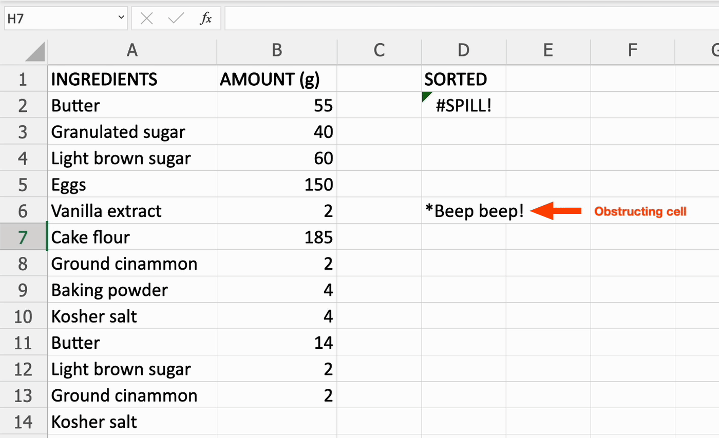
Spill range isn’t blank

Problem: The spill range is obstructed by one or more non-empty cells. 

Fix: Clear the spill range. 

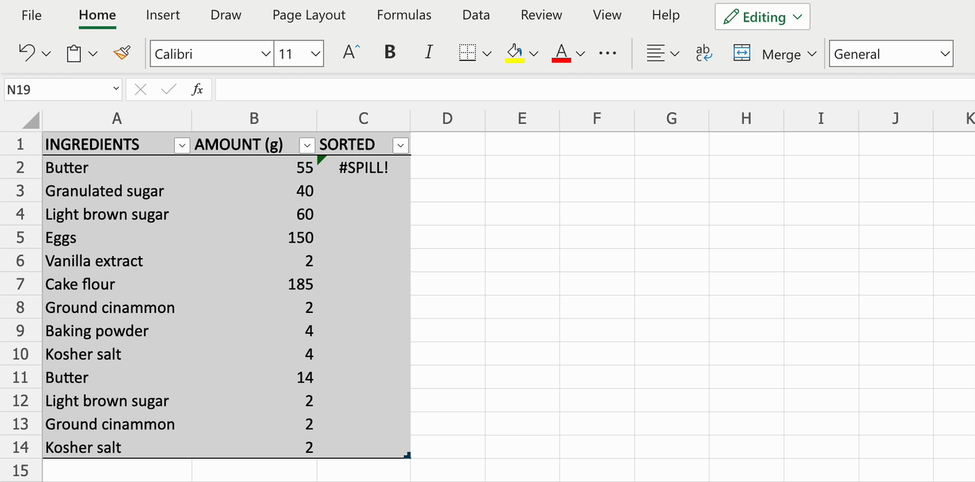
Spill range inside a table

Problem: The formula and its spill range fall within an Excel table. Unfortunately, spilled array formulas (any formula that produces a set of values that spill) aren’t supported in Excel tables.  

Formulas that are currently returning arrays that are successfully spilling can be referred to as  spilled array formulas.

Fix #1: Convert the table to a range. Here’s how to do this. 

1. Click any cell within the table. 

2. From Excel’s main menu bar just above the ribbon, select Table Design. (This menu option will only appear after you click a cell within the table.)

3. From the ribbon, select Convert to Range. 

Note: If you’re using the desktop app, your menu and ribbon may appear different from the video above, but the steps will be the same. 

Fix #2: Alternatively, you can move your formula outside the table.

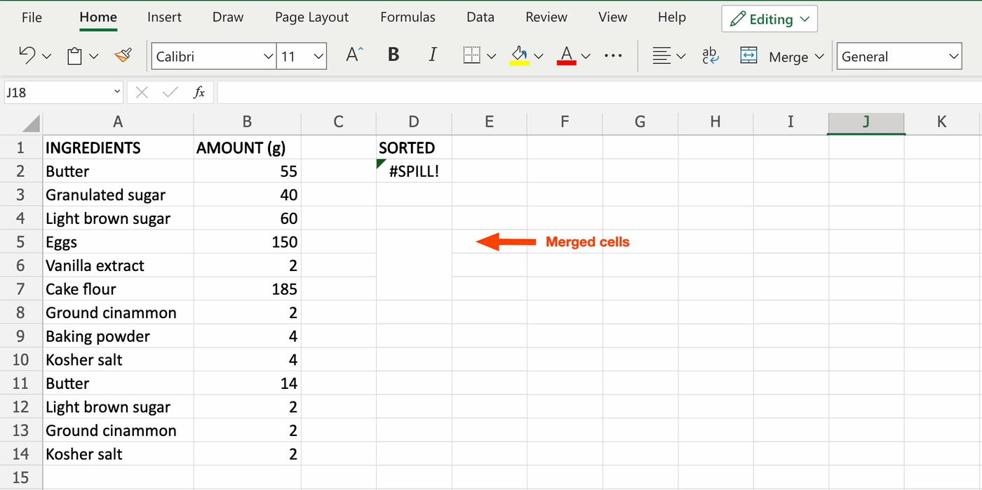
Spill range has merged cell

Problem: Two or more cells within the spill range are merged. 

Fix: Unmerge the cells within the spill range.

How to fix a #VALUE error in Excel 

A #VALUE! error in Excel occurs when either:

The #VALUE error can be vague, making it difficult to find the root of the problem. Here’s how to troubleshoot the most common sources of #VALUE errors. 

Note: You may need to apply more than one troubleshooting tip to fix your particular error. 

A mathematical formula references text

Problem: The formula uses math operations such as add (+) and subtract (-), but one or more of the cells to which the formula refers includes text. 

Note: Formulas with math operations can only calculate numbers. 

Fix: Use a function instead of a formula. (A function is a preset formula that’s already programmed into Excel, whereas a formula is any equation written by a user. In other words, all functions are formulas, but not all formulas are functions.) The beauty of functions is that they automatically ignore most text values and only calculate numbers. 

For example, the function =SUM(B2,B11) would ignore the text in cell B11 and only calculate numbers. 

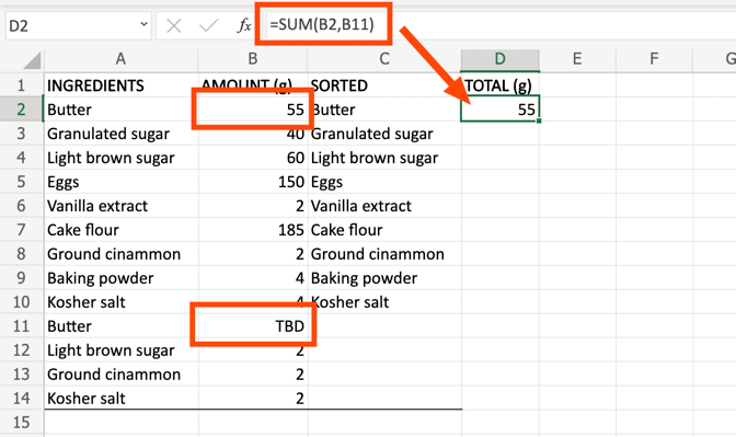
Note: Since this function ignores any text strings and doesn’t automatically notify you of these omissions, the function’s answer may be misleading. There are approximately a zillion advanced formulas you could write to work around this—but that’s an article for another day. 

One or more cells contain hidden spaces

Problem: One or more referenced cells contain hidden spaces. The cell will appear blank, but it actually contains a space. 

Fix: Find and remove any hidden spaces in the reference cells.

1. Select and highlight the range of cells to which your formula is referencing. 

2. From the Excel ribbon, click the magnifying glass icon in the ribbon, then click Replace.

3. From the top of the Find and Replace pop-up window that appears, select Replace. 

4. In the text field beside Find what: add at least one space. (If you have cells with multiple joined spaces, this search term will find them.) 

5. Leave the text field beside Replace with: empty.

6. Select Replace All. 

How to fix #REF in Excel 

A #REF! error in Excel occurs when a formula references a cell that no longer exists. Here’s how to troubleshoot the most common sources of #REF errors. 

Reference cell has been deleted 

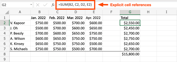
Problem: The formula uses explicit cell references (where each cell referenced is separated by a comma), but one or more of the cells referenced has been deleted. This is the main reason why Excel does not recommend using explicit cell references. 

Fix #1: If reference cells were accidentally deleted, immediately undo the action. 

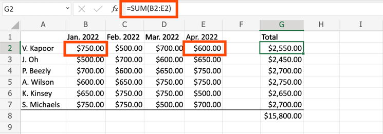
Fix #2: Update the formula so that it references a range of cells instead of using explicit cell references. For some inexplicable reason, Excel is able to compute a formula with cell ranges—even if one or more reference cells are missing.

In the example below, cell B2 is the first cell and cell E2 is the last cell, so the updated formula is =SUM(B2:E2). 

A formula uses relative references

Before we troubleshoot this error, let’s talk about relative references. 

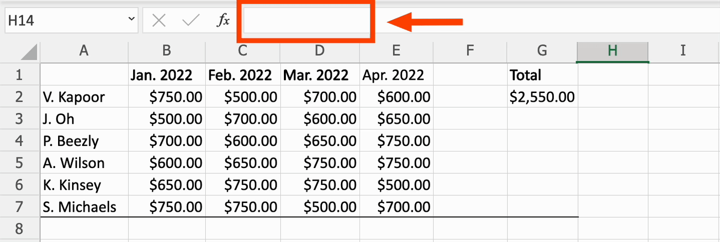
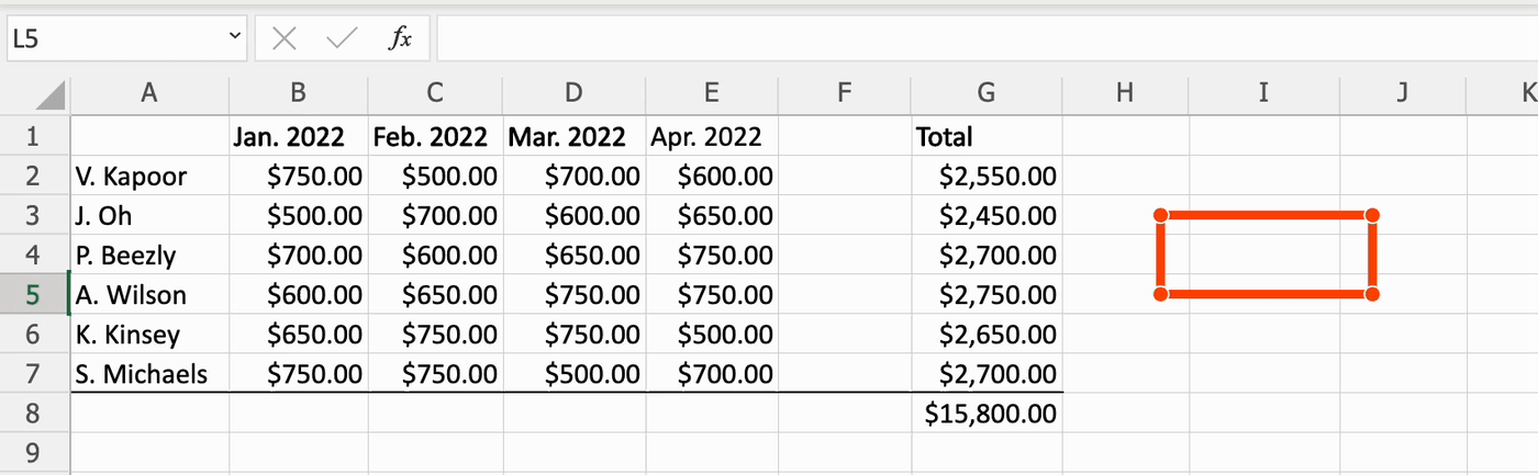
A relative reference means that the data used (or referenced) is relative to the location of the cell where the formula was inputted. For example, if the formula =SUM(B2:E2) from cell G2 is copied to cell G3, Excel will assume it should add the sum of all cells ranging from columns B to E within row 3 (or the same row that the formula has been pasted into). Whenever a formula containing a relative cell reference is copied and pasted somewhere else in a worksheet, that reference will automatically change. 

Now back to the problem at hand. 

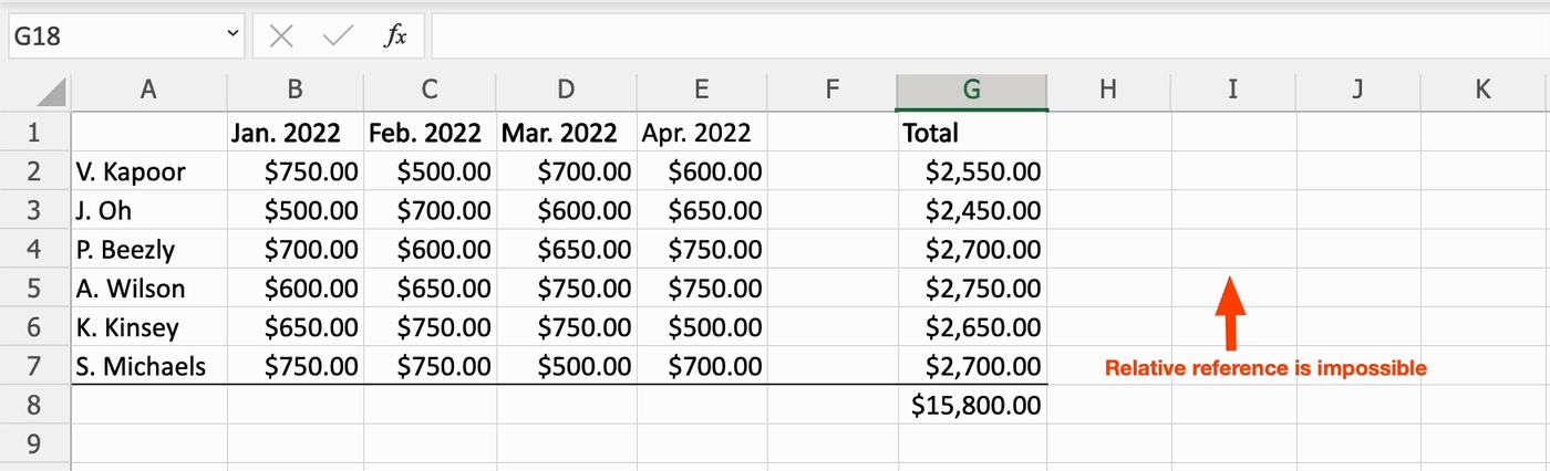
Problem: A formula with relative references has been copied to another area of the worksheet, or another worksheet altogether, but the reference is impossible.  

For example, if the formula =SUM(G2:G7) is copied to cell I4, Excel assumes you want to add the six cells immediately above cell I4. In this example, that’s impossible as there are only three reference cells available. 

Fix: Update your formula to include absolute references. This allows the formula to maintain the original cell references if the formula is copied to another cell within the same worksheet. To make the cell reference absolute, include a dollar sign ($) immediately before each column letter and row number that you want to stay the exact same, directly in the formula. 

For example, to make =SUM(G2:G7) absolute, it would become =SUM($G$2:$G$7).

How to fix a #NAME error in Excel

A #NAME! error in Excel appears when there’s an error in the formula name. Here’s how to troubleshoot the most common sources of #NAME errors. 

Formula name contains a typo 

Problem: The name of the function within the formula contains a typo. 

Fix: Update the function name.  

The best way to avoid typos in function names is to use Excel’s handy Formula Wizard. As you start typing the function name, Excel will automatically suggest a list of function names containing the same letters. 

Formula name is wrong 

Problem: The function name refers to a formula that doesn’t exist, or it exists under a different function name. 

For example, the function “ADD” does not exist in Excel (you’re probably looking for “SUM”), so any formula containing “ADD” would produce a #NAME error. 

Fix: Find the right formula name, and update the formula accordingly. Here’s how to find a list of every possible function in Excel. 

1. Select Formulas from the menu bar. 

2. To explore all possible functions, select Insert Function from the far-left in the ribbon. A Formula Builder window will pop out on the right side of the screen and show you Most Recently Used functions along with All possible functions immediately beneath that. 

3. Select the function you want, and click Insert Function.

4. While in the Formula Builder, update the cell(s) to be referenced. (The cell fields required will vary based on the function inserted.)

Troubleshoot even more spreadsheet errors 

If you spent most of your life using Microsoft, but you’ve finally seen the Google light, you’ll be thrilled to know that many Google Sheets errors are more or less the same. (One exception is the #SPILL error, which will often pop up as a #REF error in Sheets. The solutions are the same, though.)

Regardless of the app you’re using (I won’t judge), bookmark this cheat sheet, and enjoy your error-free spreadsheeting.

Related reading: