
Raise your hand if you’ve ever entered data into Excel and immediately asked yourself, “Wait. Didn’t I already type that?” Whether it’s an import error or human error, duplicate data makes your spreadsheets less useful.

Here’s how to find duplicates in Excel, so you can delete them yourself. Plus, I’ll show you two ways to find and remove duplicate rows in one fell swoop.
How to find duplicates in Excel
If you simply want to find duplicates, so you can decide whether or not to delete them, your best bet is to highlight all duplicate content using conditional formatting.
-
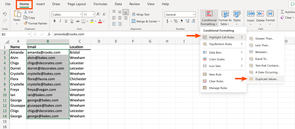
Select the data you want to check for duplicate information. Then, from the Home tab, select Conditional Formatting > Highlight Cell Rules > Duplicate Values.
-
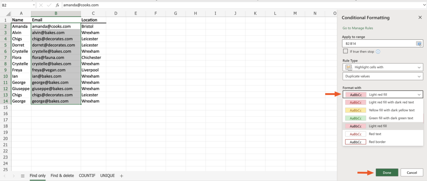
From the Conditional Formatting window that appears, click the dropdown menu under Format with to select the color scheme you’d like to use for highlighting duplicates. Then click Done. (Tip: Choose a high contrast color scheme, such as Light red fill, to improve readability.)
-
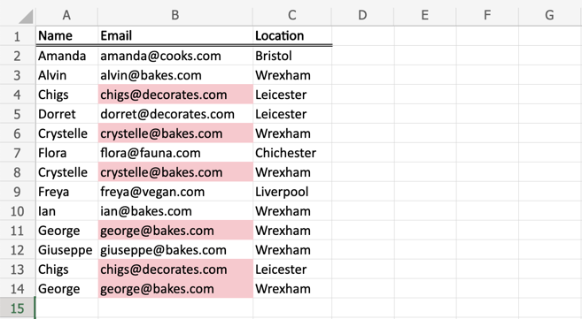
You can now review the duplicate data and decide whether you need to delete any redundant information.
How to remove duplicates in Excel
If you’d like to find and delete duplicates in Excel without manually reviewing them first, you can accomplish this in one of two ways.
Use the remove duplicates feature in Excel
-
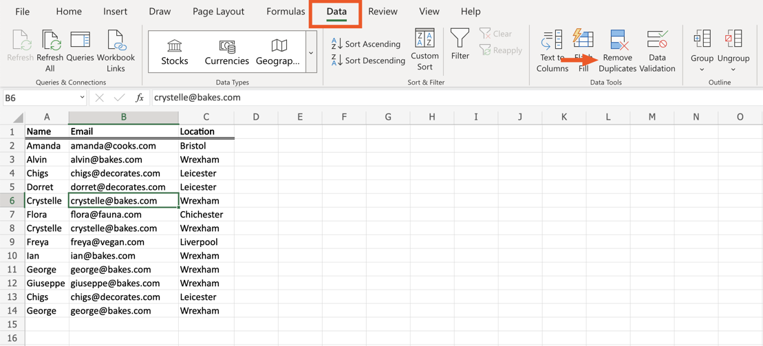
Click any cell that contains data. Then, select the Data tab > Remove Duplicates.
-
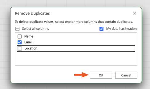
From the Remove Duplicates window that appears, select which columns you’d like to include in your search for redundant data. Click OK. (The Remove Duplicates tool will permanently delete duplicate data, so it’s a good idea to copy the original data to another worksheet for backup.)
-
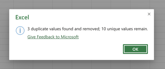
Excel will let you know how many duplicate values were removed.
Use the UNIQUE function in Excel
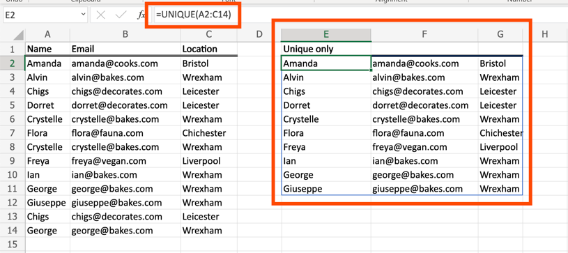
In Excel, the UNIQUE function returns unique values (i.e., data that’s not duplicated) from a list or range. The only caveat is that this will not replace your existing data. It exists within the same spreadsheet as the original source of data.
To get a unique list of values, select an empty column of your spreadsheet. Then input the UNIQUE function using the cell range you want to scan for duplicates, leaving behind only unique values. For example, =UNIQUE(A2:C14).
Related reading:
This article was originally published in June 2019 by Justin Pot. The most recent update was in October 2022.
Need Any Technology Assistance? Call Pursho @ 0731-6725516


