
Let’s say you have a list of email addresses that you collected through a form on your website. You want to know how many email addresses you received, but you’re worried that someone may have filled out the form twice, which would inflate your numbers.

When you’re working with large amounts of data in a spreadsheet, you’re bound to have duplicate records. Whether it was human error or robots that put them there, those duplicates can mess with your workflows, documentation, and data analysis.
Google Sheets now offers a built-in feature to remove duplicates. Here, we’ll show you how to remove duplicates in Google Sheets using that tool and then offer some more advanced alternatives if that doesn’t do the trick.
Follow along with this tutorial by trying the instructions for yourself in this demo spreadsheet. Be sure to click File > Make a copy first.
Remove Duplicates from Google Sheets Using the Built-In Feature
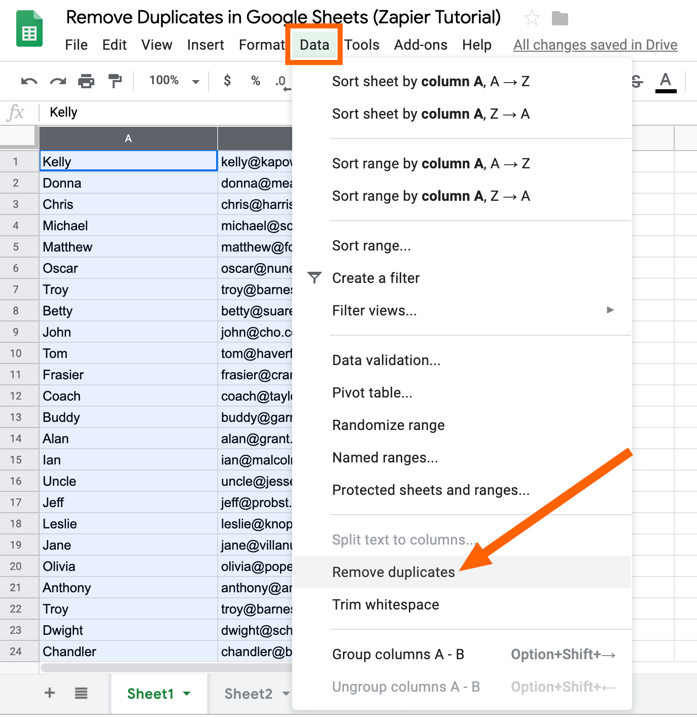
The built-in feature offers the basic functionality of removing duplicate cells. To do so, highlight the data you’d like to include, and click Data > Remove duplicates.
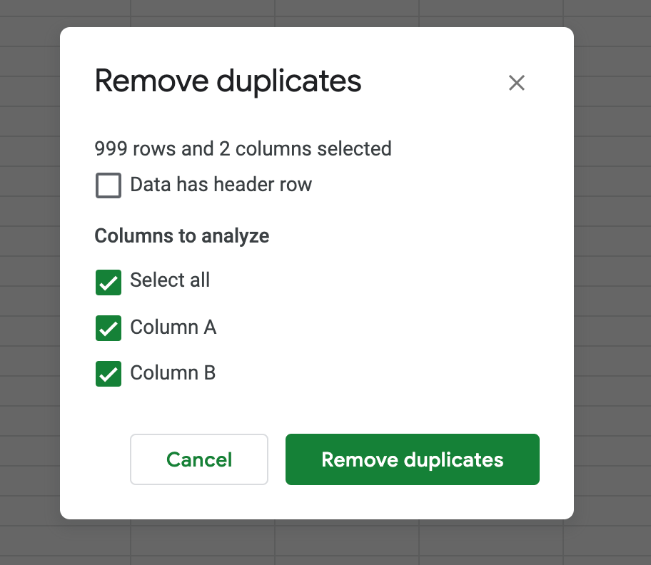
At that point, you’ll have the option to select if the data has a header row and confirm what range you’d like to work with.
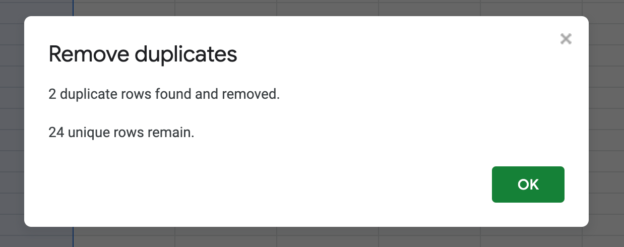
Once you’ve made your selections, click Remove duplicates, and the job is done. It’ll let you know how many duplicates were removed.
Remove Duplicates from Google Sheets Using a Formula
If you want to remove duplicates but keep the original data where it is, you can use a formula called Unique. It allows you to find the records that are unique—i.e., not duplicated—and then get rid of the rest.
Remove duplicates from within a single column
Let’s say you want to pull out only the unique email addresses from Sheet1 in our demo spreadsheet.
Step 1
Decide where you want your de-duplicated data to live—that is, your clean data set after you’ve removed the duplicates. In our example, we created a new sheet for this purpose: Sheet3.
Click into the cell at the top left of the sheet. (If you choose to put the data elsewhere, be sure there’s enough space below and to the right of the cell you select because the formula will overwrite whatever is currently there.)
Step 2
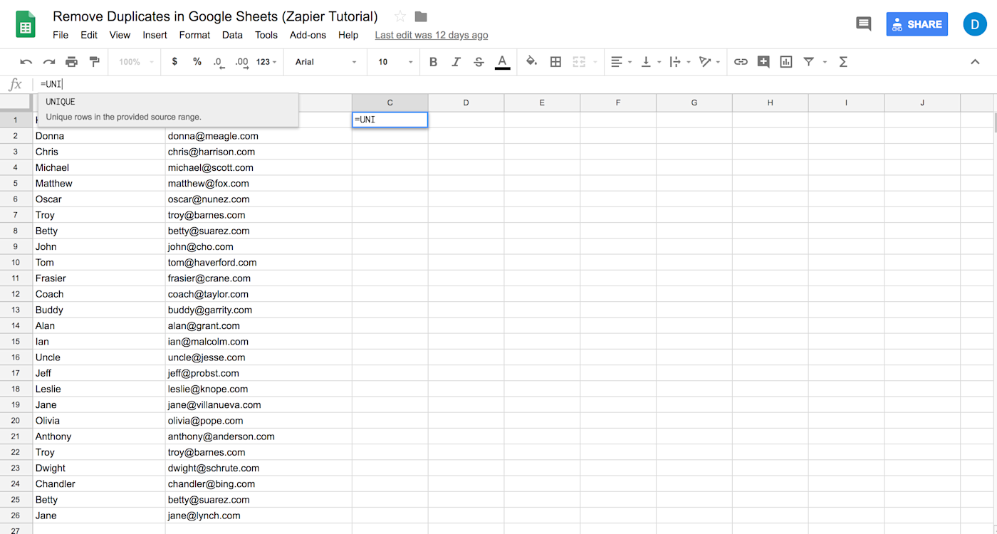
Type =UNIQUE( into the formula bar (the correct formula appears once you start typing the word).
Step 3
Go back into the sheet with your data (Sheet1). Select the column from which you want to remove duplicates by clicking on the letter at the top of the column (in this case, B). Notice that the formula automatically adds the range for you.
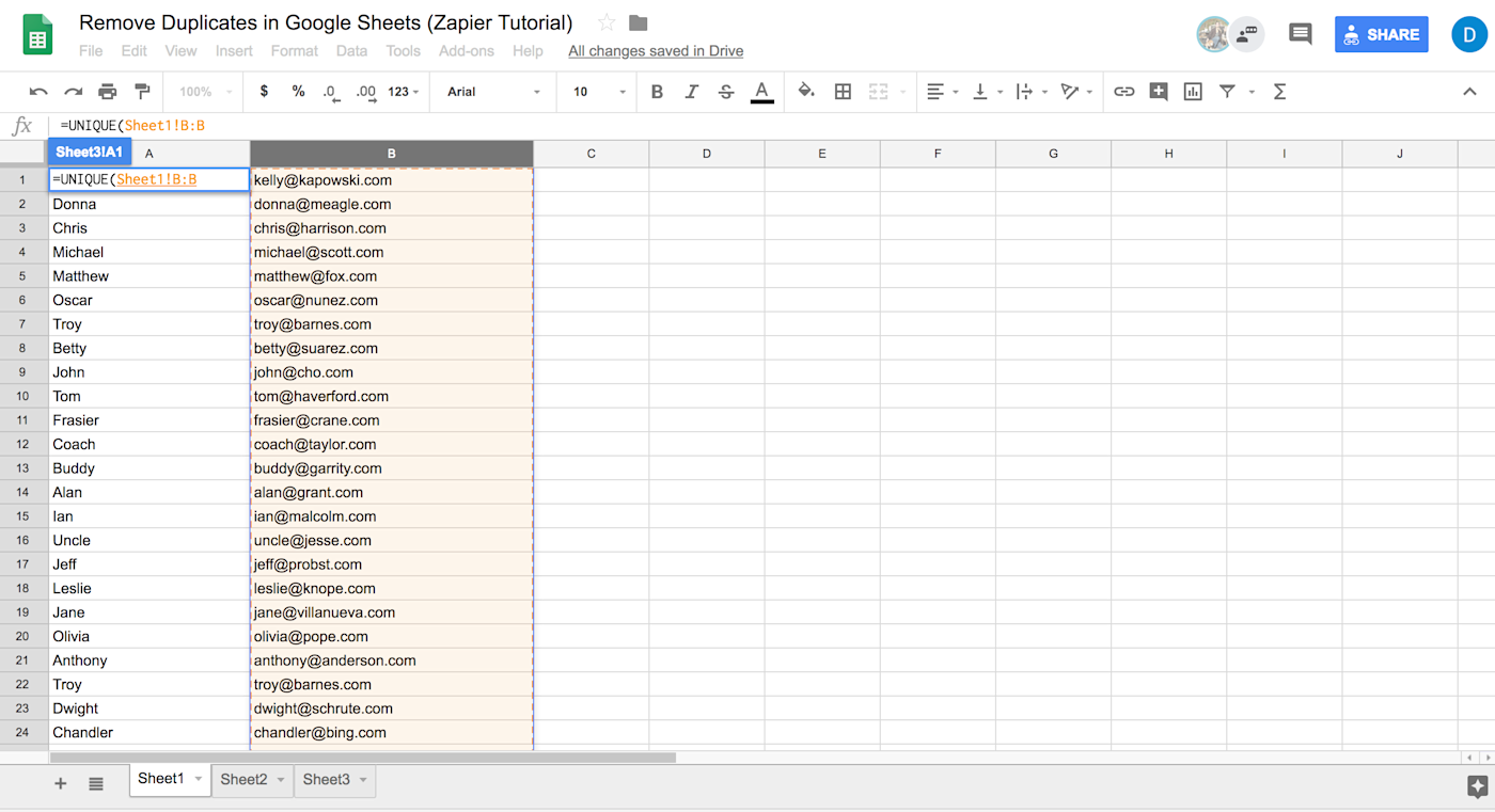
Now all you need to do is type the end parenthesis, ), to complete the formula. Your formula will end up looking like this:
=UNIQUE(Sheet1!B:B)
Step 4
Press enter, and the unique records from the selected column will appear, starting in the cell where you entered the formula.
Step 5
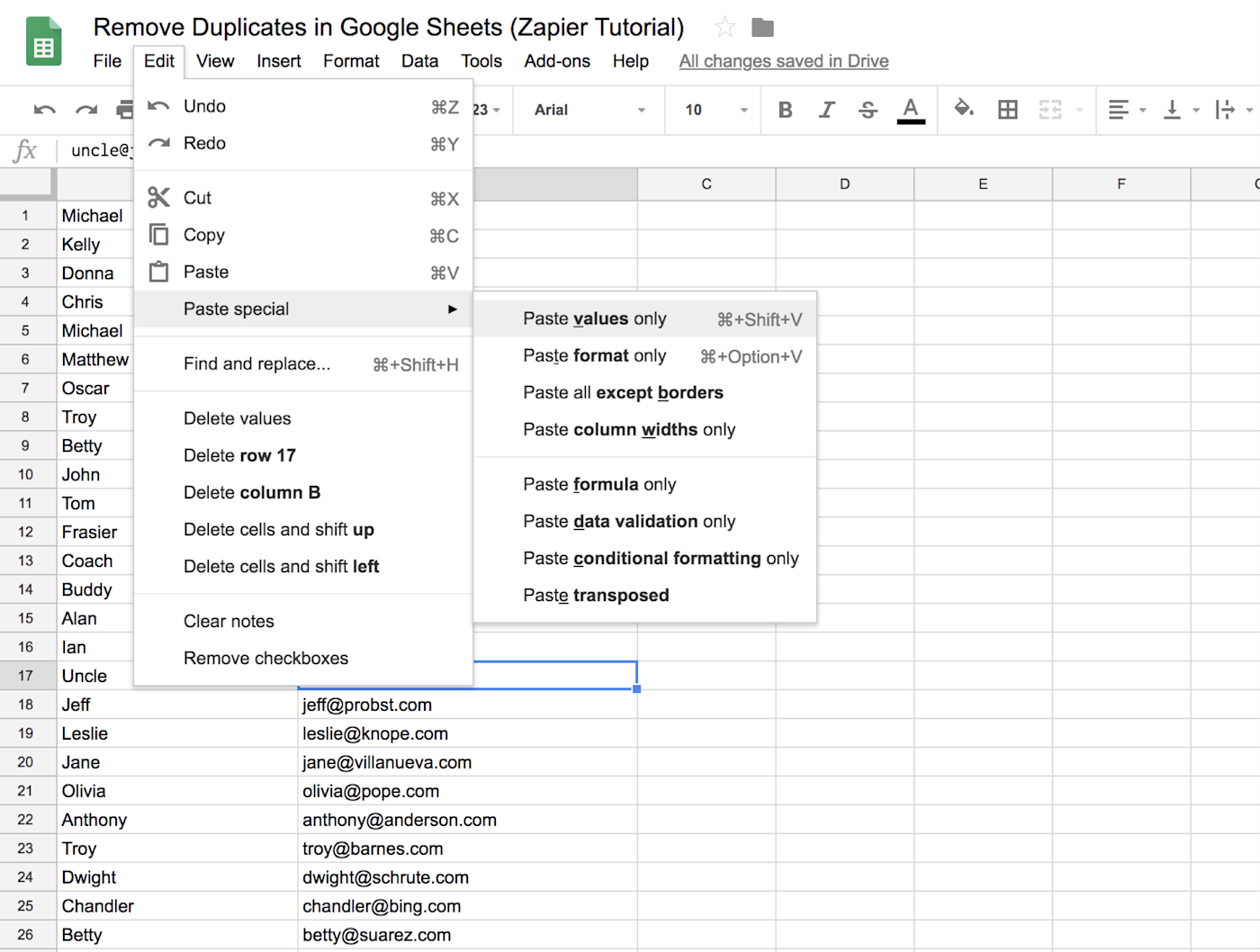
Now you can use that de-duplicated data anywhere you want. Be sure that if you copy and paste into another spot in Google Sheets, you choose Edit > Paste special > Paste values only. Otherwise, you’ll end up copying the formula instead of the results.
Remove duplicate rows from within a sheet
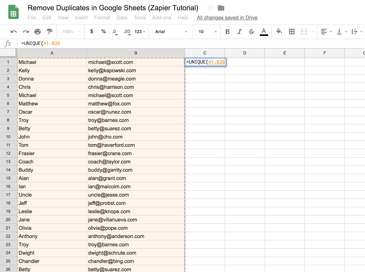
The process for removing duplicate rows is similar, the only difference being the range of cells you select. Follow the process above, but for Step 3, select the rows from which you want to remove duplicates.
In our example spreadsheet, highlight rows 1-26 of Sheet1 in order to delete any duplicate entries.
To include specific rows that aren’t next to each other, select each row by using the command button on a Mac or ctrl on Windows.
Remove Duplicates from Google Sheets Using an Add-on
The formula method is simple, but what if you want to address issues with duplicates beyond simply deleting them, such as:
-
Identifying duplicates (not deleting them)
-
Deleting both instances of duplicated data
-
Comparing data across sheets
-
Ignoring a header row
-
Automatically copying or moving uniques to another location
-
Clearing any duplicate data or removing an entire row where there are duplicate data
-
Ignoring letter casing (e.g., finding duplicates even if one is uppercase and one is lowercase)
If you need to address any of those situations—or if you have a more robust data set than in the example above—use the Remove Duplicates add-on instead.
Install the add-on
First, install the add-on. Click Add-ons from the Google Sheets toolbar and choose Get add-ons. Search for and select the add-on called “Remove duplicates” offered by Ablebits.com (free for 30 days; $59.60 for a lifetime subscription or $33.60 annually).
Authorize the add-on when prompted. Follow the steps, and the add-on will immediately be added to your account.
If you use multiple Google accounts, such as a personal account and a work account, install the add-on separately for each account.
Now when you click Add-ons, hover over Remove Duplicates, and you’ll see two choices:
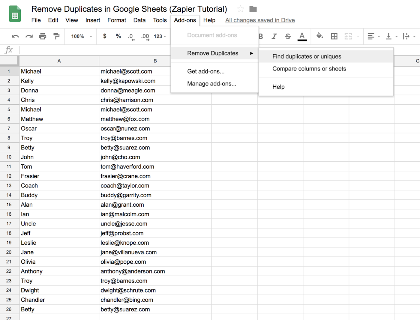
Find duplicates or uniques
If you choose the first option, you’ll be able to find either duplicates or unique entries and take a number of actions on them.
Step 1
Choose the range of cells you want to search. The add-on will start by auto-detecting what range you might want to look at, but you can override that by manually typing in cell numbers or clicking the spreadsheet icon in the text field and selecting the cells on the sheet itself.
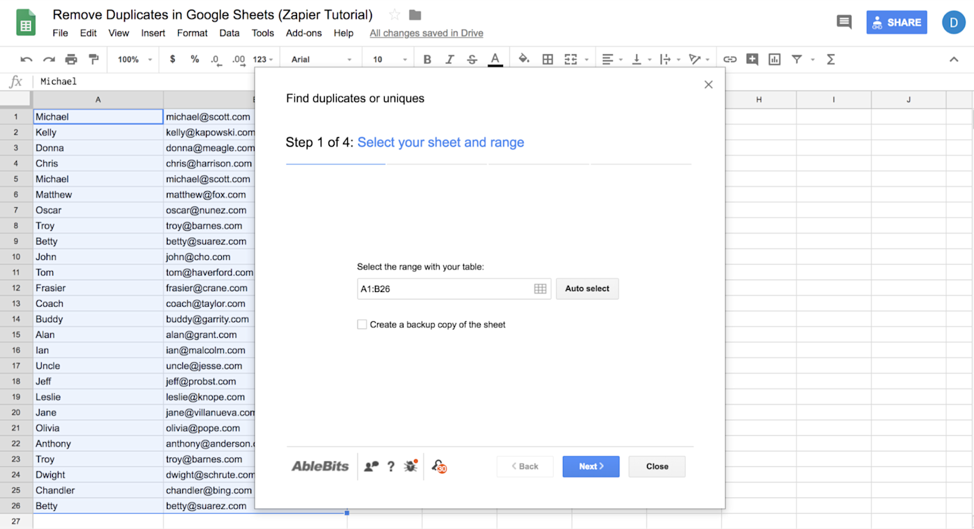
In our example spreadsheet, choose columns A and B of Sheet1.
If this is your first time using the add-on, or if you think you might use this data again, select “Create a backup copy of the sheet” (within this view) to be sure you don’t lose any valuable data. The version history feature of Google Sheets will always allow you to revert, but better safe than sorry.
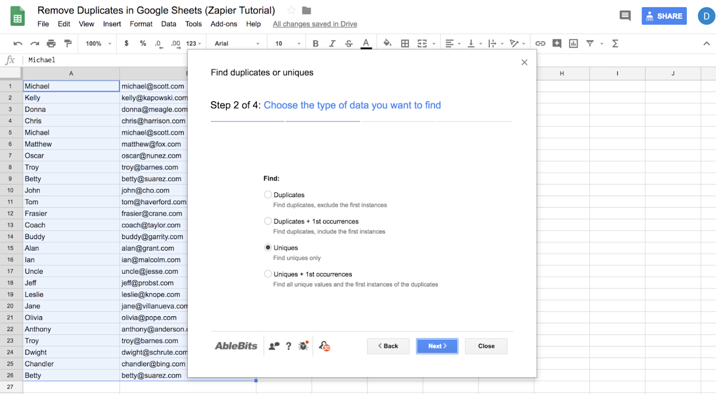
Step 2
Decide what type of values you want to find. You can choose uniques only, mimicking the =UNIQUE( formula, or you can find duplicates.
In either case, you also have the option to find the first occurrence of duplicates. Why would you choose to do that? Say you were trying to determine who in your office spoke a language that no one else in the office spoke. If you had all the entries in a spreadsheet (name in column A, language in column B), deleting only the second occurrence of the duplicates wouldn’t help you because you’d still be left with languages spoken by more than one person. But if you delete the duplicates including the first occurrence, you’d be left with languages that only one person spoke.
Step 3
Now you’re going to confirm a few details. For example, do you want to skip the empty cells? Does your range have a header row that you want to ignore? Do you want to ignore uppercase and lowercase variations?
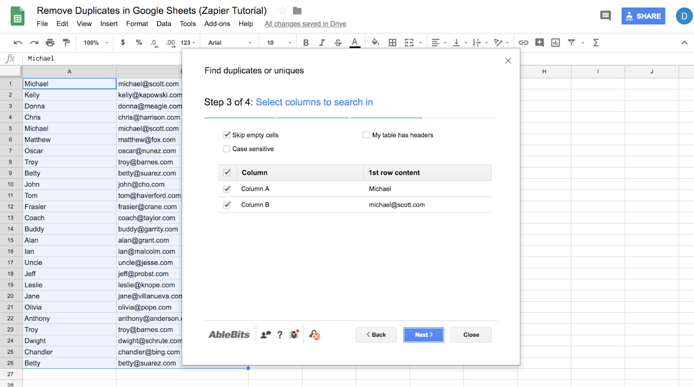
Feel free to play around with this add-on. If at any point you change your mind about your selections, you can always click Back.
Step 4
Now you have options for what you can do with the values found in the previous steps. The ones we find most useful are:
-
Fill with color. This allows you to identify duplicates or uniques without taking any action on them. That way you can highlight for yourself and your team whenever there’s duplicate data.
-
Copy to another location. This allows you to save your current data as is and move the new data either within the current worksheet (“Custom location”), to a new worksheet within the current spreadsheet, or even to an entirely new spreadsheet.
-
Clear values or delete rows within selection. This is particularly helpful if you want to delete uniques and be left with only duplicates.
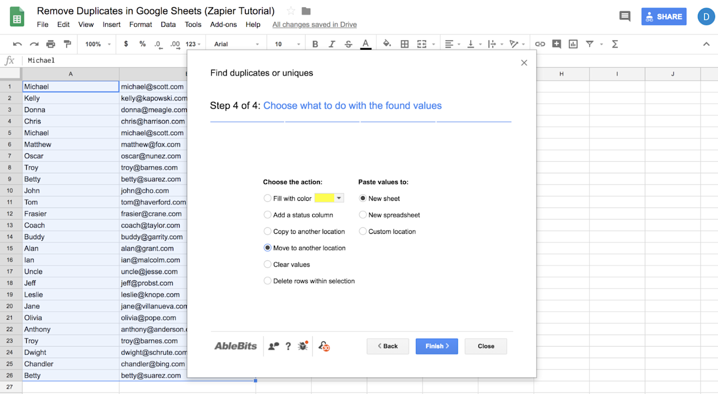
Step 5
Click finish, and that’s that.
Compare columns or sheets
If you want to compare two columns within the same worksheet or you want to compare data across two worksheets, choose Compare columns or sheets when starting the add-on.
Step 1
First, select the sheet where your first data set originates. If you only have one sheet, you still need to complete this step.
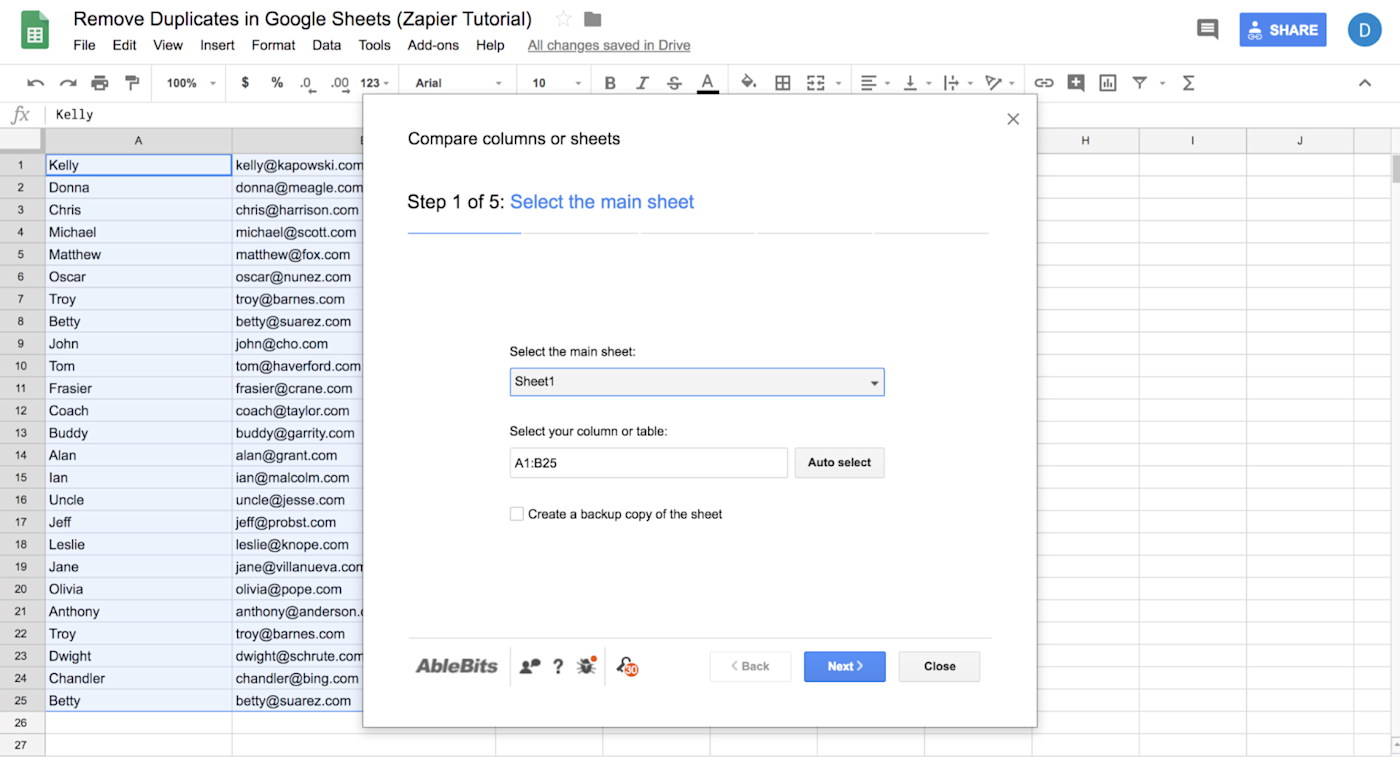
In the same step, select your range. It can be an entire column or some other set of data (table).
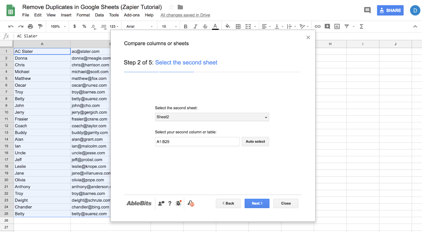
Step 2
Select the sheet and column or table that contains your second data set.
Step 3
Now choose whether you’re looking for duplicates or uniques.
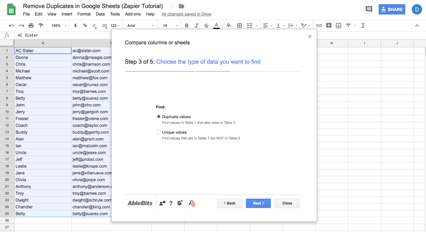
Note that the add-on defines duplicates and uniques based on which table or dataset contains them. Duplicates are values in Table 1 that also exist in Table 2. Uniques are values that are in Table 1 but NOT in Table 2.
So, if you were looking for values that are in Table 2 but not in Table 1, you’d want to go back and swap which data set you select first.
Step 4
Now, select which columns to compare.
Under “Table 1 columns,” select the columns from your first data set that you want to include in the comparison.
Under “Table 2 columns,” select from the dropdown which column from the second data set you are comparing to.
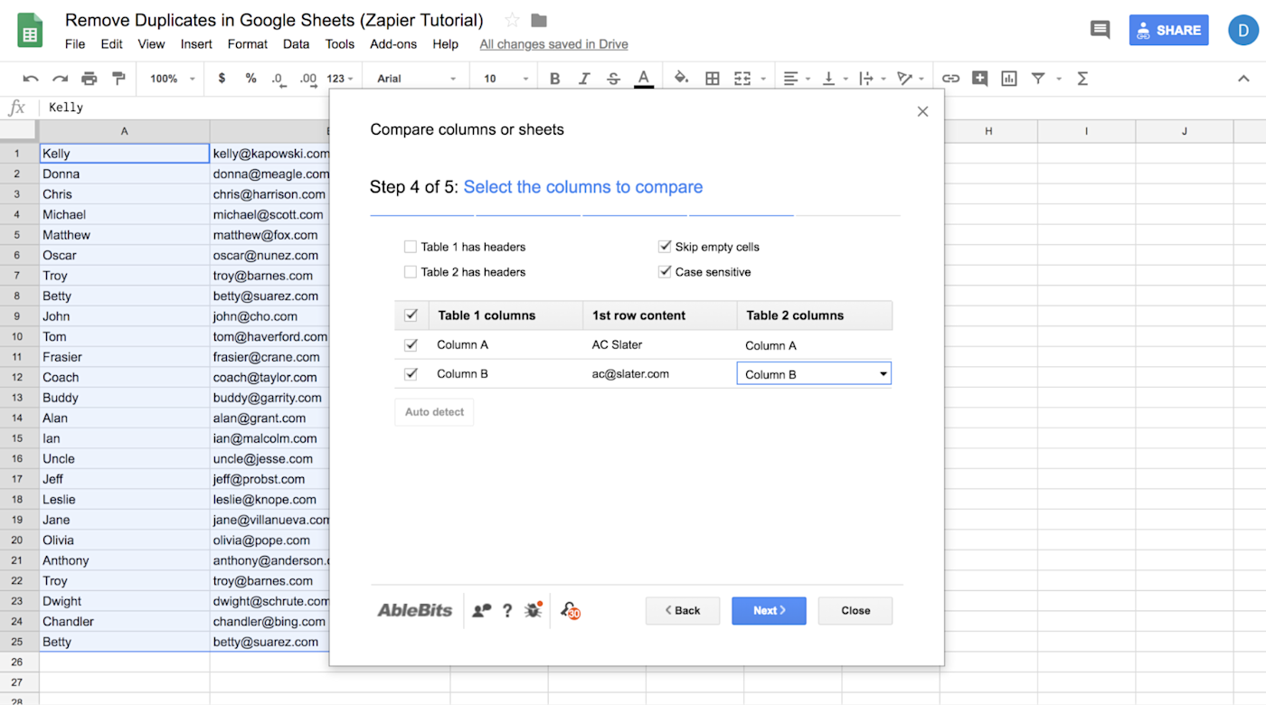
It’s possible you’ll compare apples to apples—i.e., Column A in Sheet1 to Column A in Sheet2 and Column B in Sheet1 to Column B in Sheet2. But if you’re working with two sheets that are organized differently from each other, you have the option to adjust.
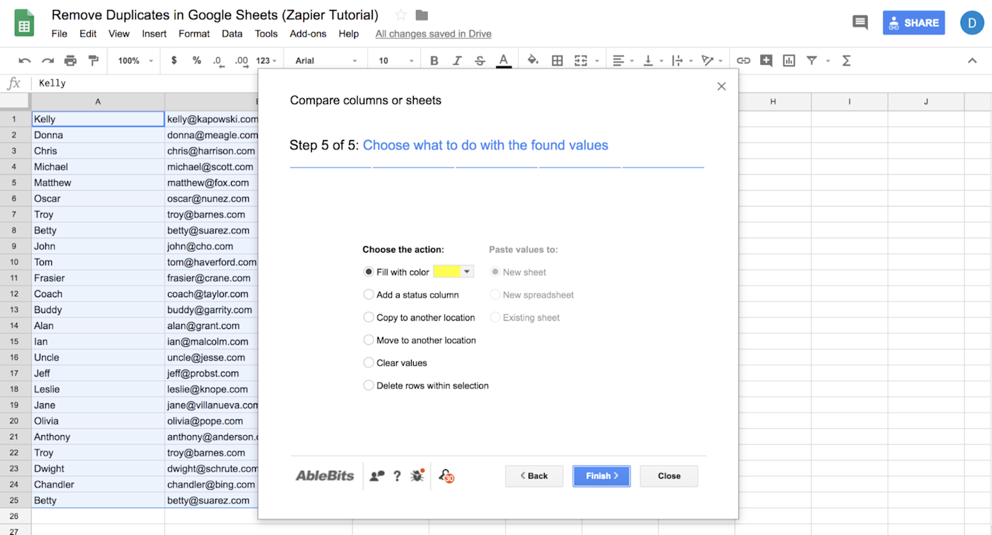
Step 5
Choose what you want to happen with the found values, and click Finish.
Take some time to play around with our demo spreadsheet, and you’ll see how easy it is to find, delete, or format duplicates—or uniques—in Google Sheets, no script required.
Need Any Technology Assistance? Call Pursho @ 0731-6725516


